Lecture 2 Solow Growth Models
This chapter deals with the specifics of the Solow Growth model. We use the neo-classical economic model as a broad framework to understand how the economies improve their living standards through capital accumulation.
The economy uses various kinds of capital. Infrastructure just one of the types of the capital the firms and household use in the economy. Yet, it is special category of capital in the way it relates to other form of factor inputs. It is special because it allows other factor inputs to be more effectively in the production process.
In this chapter, we look at the all encompassing notion of generic capital. We will start examining the exact role of infrastructure and its relationship with other types of capital in subsequent chapters. We will find that infrastructure is crucial for the capital accumulation process and engenders economic growth and economic development through myriad channels. Thus, understanding the process of capital accumulation is the crucial first step in understanding how nations becomes prosperous.
2.1 Role of Theory
The world is complex and we are constantly inundated with information and data. To make sense of the world, we need a logical framework that would allow us to see the patterns that are important.
A theoretical model is exactly this logical framework built from a set of logical propositions. A logical proposition is a simply a statement that says “if \(p\) and \(q\) holds, then \(r\) would occur”. The logical proposition says that the occurence of the \(r\) phenomenon is dependent on \(p\) and \(q\) occurring. In what follows, we will make some assumptions (akin to \(p\) and \(q\) above) and works the logical outcome (akin to \(r\) above). Good theory makes certain assumption and works out the logical propositions that follow from the assumptions.
Every theoretical model’s Achilles heel are its set of assumptions. If the assumptions can be justified, then the theory can be validated. Alternatively, empirical validation of the predicted phenomenon validates the assumptions. It is useful to think about the following aphorism attributed to George Box.
“All models are wrong, but some are useful” – attributed to the statistician George Box.
Reality is complex and it is difficult to find patterns within the weeds of reality. It is the role of a model to delineate the pithy truth that captures a crucial aspect of reality. Hence, the models are never a true representation of reality. In capturing the essence of reality and leaving out mundane details, they are wrong, yet they are a very useful for us to understand the complex world that surrounds us.
Like all other models, the neo-classical growth model is wrong, but it is extremely useful and insights gained from it have transformed millions of lives around the world. The neo-classical growth model represents work of academics like Frank Ramsey Roy Harrod and Evsey Domar, Trevor Swan and Robert Solow over three decades. This literature culminated into a Solow Growth model model (Solow 1956).
2.2 Solow Growth Model I
Assumptions
The section below explains the Solow growth model and explores the results of the model and the assumptions the results are contingent on.
There are the following two critical assumptions in Solow growth model.
constant returns to scale. The assumption asserts that the scale of production does not matter. Large and small firms work in the same way. With this assumption, we can abstract from the complication of economy as it exists and study it like it was one firm using capital, labour and technology to produce output.
Diminishing marginal product of capital. The second assumption is that the greater the amount of capital used in a production function, the less productive it is. Even though these assumptions are strong ones, it gives us a deep insight into the fundamental the process that drives economic growth. Once we have this insight, we can add other details as and when we please. In this way, these assumptions extremely empowering.
These two assumptions have been subject of much discourse and reexamining these assumptions led to the development of a new strand of growth theory called Endogenous growth theory. 7 While Endogenous growth theory explains why the living standards continue to increase in developed countries even after they become prosperous, Solow growth model still remains the appropriate framework to understand what increases living standards in developing countries.
Firm’s production Function
Most production in the economy takes place within firms. To understand the forces that drive the growth process it is fundamental that we understand how production takes places within a firm.
As we will see later on, we can extrapolate quite easily from what happens with a firm to what happens at the level of the economy under some conditions. Of course, the firms across the economy differ in an number of ways. Yet, there is something common about the way in which all firms produce. Understanding the economy through the firms is the first step in understanding the growth process. Once we got a firm grasp on this aspect, we can add other complication to the framework.
A firm uses range of factor inputs and turns it into output. We can broadly put the factor input into two different categories depending on whether they exhibit characteristics of stock or a flow. For example example, water flows when it is in a river. Conversely, water is a stock when it is in a pond. Any production process requires a combination of factor inputs that are stocks and flows.
We usually think of physical capital as a stock input, i.e., a stock of machinery. It just sits there inertly as it is. We think of human labour as flow. The third factor input into the production function are a set of ideas or technology about how to combine the capital with labour to produce a flow of output.
A firms production function thus uses a stock of ideas to combine the stock of capital and flow of labour it hires to produce a flow of output. We use the function \(F(\cdot)\) below to describe how factor inputs capital and labour are turned into output.
A firm’s production function is given by \[Y = F(K, AL)\] where \(Y\) is the output, \(K\) the capital, \(L\) the labour and the \(A\) is the set of ideas or technology that makes the worker more productive. At this stage, think of \(A\) as anything that makes the worker more productive. \(A\) and \(L\) go into the production function together because the ideas that improve productivity and human labour work together to utilise the physical capital to produce a flow of output. New ideas or technology enhances the capability of the worker and \(A\cdot{}L\) can be thought of as an effective worker. Put another way, \(AL\) represents exactly how effective a worker in using the capital \(K\) to produce a flow of output.
An economy has range of different types of firms that turn factor inputs into outputs. It is not easy to derive a production function for the whole economy. The process of deriving the production function for the whole economy is called aggregating, i.e., aggregating all the production function in the country and representing them with a grand production function which describes the relationship between economy’s factor inputs and output. The simplest form of such a production function would describe how capital and labour are combined to produce economy’s output. As one would expect, it is not easy to aggregate the production function. Though, there is a magical assumption, which if true allows us to aggregate. That magical assumption is constant returns to scale.
Lets step back for a moment and think whether we can really aggregate all the physical capital into one silo of capital. That is, can you add screwdrivers with cranes to come to one single measure of total physical capital in the economy. The answer to depends on the purpose behind aggregating the capital. If we wanted to aggregate capital for the purpose of discovering what the true value of capital in the economy is then that would be an arduous exercise. That though is not our objective. Our objective in stead is to understand the processes that create physical capital and flow of output the physical capital in turn creates. As we see below, the stock of new capital in the economy is created from the flow of non-consumed output. Given that our objective is to understand how to influence the flow of goods in order to expand the productive capacity of the economy, aggregating for this purpose is easier.
Returns to Scale
There are three possible types of returns to scale: increasing returns to scale, constant returns to scale, and diminishing (or decreasing) returns to scale.
If output increases by the same proportional change as all inputs change then we say that the production function exhibits constant returns to scale.
A production function exhibits decreasing returns to scale when output increases by less than that proportional change in all inputs. Similarly, a production function exhibits increasing returns to scale is when output increases by more than the proportional change in all inputs.
Example: Imagine a small coffee shop with 5 barista and 5 espresso machine. The shop produces produces 200 espresso a day. The scale of the production expands and now there are 10 baristas and 10 espresso machines. If the coffee shop now produces 400 espresso a day, we would conclude that the coffee shop’s production function has constant returns to scale. If the coffee shop produces more than 400 espresso, then it has increasing returns to scale and if it produces less than 400 espresso, it has decreasing returns to scale.
Economy’s Production Function
If firms in the economy have constant returns to scale, then economy’s production function can be estimated by a representative firm’s production function.1
Economy’s production function:
\[\begin{equation} Y = F(K, A L) \tag{2.1} \end{equation}\]
where \(Y\) is economy’s output, \(K\) and \(L\) are that total available capital and labour in the economy. \(A\) represents the set of ideas that determine the productivity of the typical worker in the economy.
\(A\) is all ideas related to science, management or society in general that increase the productivity of the typical worker. For instance, prevalent discrimination on the basis of sexual orientation, gender and race can reduce the value of \(A\) both at the level of the firm and the level of the economy. Another example of \(A\) is the idea of just-in-time manufacturing also knows a short-cycle manufacturing. \(A\) is often intangible and difficult to quantify. It interpretation is difficult, yet given the critical role it plays in ensuring that the economy grows, its interpretation can be extremely rewarding.
If the production function has constant returns to scale, its output changes by the same proportion as its input. If we were increase the inputs by a arbitrary factor \(\lambda\), the it would follow from (2.1) that \(\lambda{Y} = F(\lambda{K}, \lambda{AL})\). Since \(\lambda\) is an arbitrary constant, we can set it to \(\lambda\) such that \(\lambda=\frac{1}{AL}\) and get \(\frac{Y}{AL} = F \left(\frac{K}{AL}, 1 \right)\), which can written as \(\frac{Y}{AL} = f \left(\frac{K}{AL} \right).\) or
\[\begin{align} y=f(k) \tag{2.2} \end{align}\]
The left-hand side of (2.2) is output per-effective worker \(\left(y=\frac{Y}{AL}\right)\) and the right hand side is a function of capital per-effective worker \(\left(k=\frac{K}{AL}\right)\). The production function simply states that it is the capital per effective worker that key determinant of how the production process works. We can write (2.2) as \(Y=AL\cdot{}f(k)\). It says that we if we increase the capital per effective worker, the total output produced by the firms in the economy increases.
We can also write the production function in a way so that output per worker or income per worker is on the left hand side, i.e., \(\frac{Y}{L}=Af\left(\frac{K}{AL}\right)\). The production function written this way tells us that \(A\) impacts \(\frac{Y}{L}\) through two distinct channels. \(A\) has a direct impact on \(\frac{Y}{L}\) and an indirect impact through \(f\left(\frac{K}{AL}\right)\) by changing the capital per effective worker within it. If \(A\) increases, \(\frac{Y}{L}\) increases due to the direct impact and decreases due to the indirect impact that goes through \(f\left(\frac{K}{AL}\right)\). That raises the question of which impact would dominate and whether \(\frac{Y}{L}\) would increase or decrease if \(A\) increased.
Turns out that the direct impact would dominate if there if firms in the economy have accumulated sufficient capital and the assumption of diminishing marginal product of capital holds. At high levels of capital accumulation, the marginal impact of reduction of \(k\) by an increase in \(A\) is really small and the direct impact dominates.8 An increase in \(A\) would thus have a net impact of increasing the output per worker in most cases.
Goods Market Equilibrium
In a closed economy with no export or import and no government, the total income or output of the economy is either consumed or saved. The total output is composed of two kinds of goods. Consumption goods and investment goods. We know from national income accounting that an economy’s income and output have to be identical. This is because all the proceeds from the output being sold in the markets go to the denizens on the economy. Hence, all output becomes income.
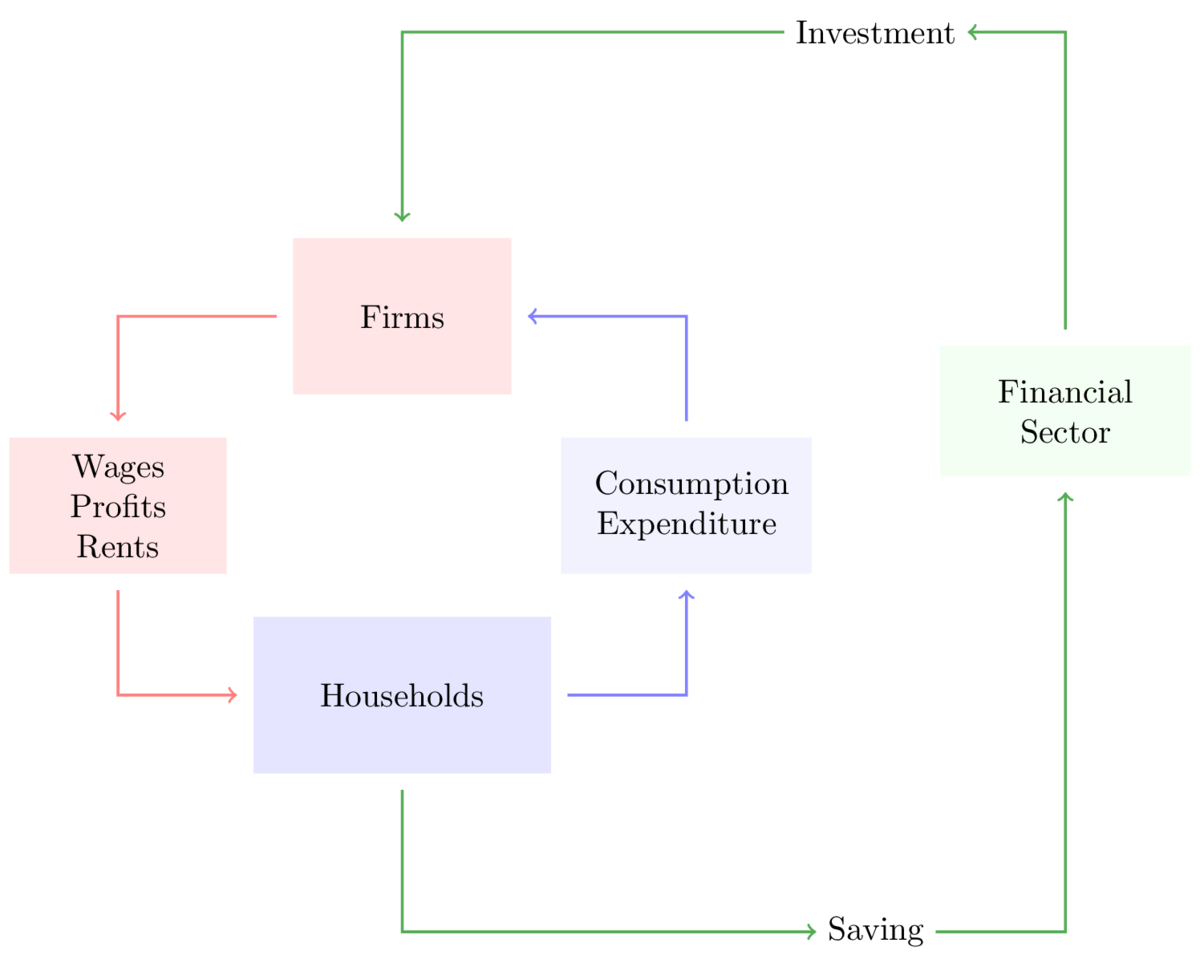
Figure 2.1: Flow of funds in the economy
If people consume \((1-s)\) proportion of their income \(Y\), then the total consumption in the economy is \(C = (1-s)Y\) and the total saving is \(S=Y-C=sY\). The output in the economy is composed of either consumptions goods or investment goods.
\[Y {~\equiv~} C+S {~\equiv~} C + I \]
It follows that saving equals investment in the economy
\[S {~\equiv~}I\]
The equation above simply states non-consumed output becomes investment through the saving-investment channel.9 This equation represents the financial sector, which is responsible for sweeping up all the saving in the economy and allocating it to the entrepreneurs who need to increase their capital stock through the process of capital accumulation. The saving-investment channel represents all the non-consumed output that is invested in the economy. If either either saving is greater or lesser than investment, then it represents the smaller of the two amounts. In countries where the financial sector is not developed, people save by putting their money below their pillow. In that situation, this equation represents the non-consumed output that is actually invested.
Investment
All machinery depreciates over time and resources have to spent in order to keep it in working condition. Every year a certain proportion of the current capital stock needs to be replaced. Any investment that is made it is divided up between capital accumulation and depreciation.
If \(\delta\) proportion of current capital stock needs to replaced every year then an economy with capital stock \(K\) will require to spend \(\delta{K}\) to keep it in working order. The net-investment \(I\) in this case is the investment left over after depreciation \(I = \Delta{K} + \delta {K}\). It follows that the change in capital stock is given by \(\Delta {K} = I - \delta{K}\).
Fundamental equation
The non-consumed output of the economy can be transformed into either depreciation or net investment. Another way to writing the same things is \(\Delta{K} = sY - \delta{K}\). This states that the new capital stock added to the economy is simply total saving \(sY\) minus the depreciation \(\delta{K}\). If divide both sides by \(K\), we write it as
\[\begin{equation} \frac{\Delta{K}}{K} = s \left(\frac{Y}{K}\right) - \delta. \tag{2.3} \end{equation}\]
\(\frac{\Delta{K}}{K}\) is growth of capital \(\frac{Y}{K}\) is total saving capital stock ratio. We will call equation (2.3) the fundamental equation because it describes the fundamental process of capital accumulation process in the Solow growth model. It simply states that the capital stock of the economy increases if the total saving capital stock ratio is greater than the depreciation rate.
Steady State
We can see from equation (2.3) whenever \(\frac{sY}{K}\neq{\delta}\), the capital stock of of the economy is only increasing or decreasing. Steady-state is simply a situation where the capital accumulation process stops, i.e., \(\Delta \left(\frac{K}{L} \right)=0.\) By imposing the condition \(\Delta \left(\frac{K}{L} \right)=0\) on the equation (2.3) above, we get the following steady-state condition.
\[\begin{equation} \frac{Y}{K} = \frac{\delta}{s} \tag{2.4} \end{equation}\]
The steady-state condition states that the output-capital ratio should be equal to the ratio of the depreciation rate and the saving rate. Looking at the production function it should be clear that for each capital stock level, there is unique output. Hence, for each \(K\) there is an unique \(\frac{Y}{K}\), which falls as \(K\) increases.10 The steady state condition in essence states that the output of the economy is determined by the \(\frac{\delta}{s}\). The steady-state condition states that countries with high \(\frac{\delta}{s}\) ratio will have high \(\frac{Y}{K}\) ratio and low total output \(Y\). Similarly, countries with low \(\frac{\delta}{s}\) ratio will have high total output \(Y\).
Dynamics
If \(\frac{sY}{K}>\delta\), \(\frac{\Delta{K}}{K}>0\), i.e., the economy accumulated capital in that period. A higher \(K\) would mean a lower \(\frac{Y}{K}\) next period, which would mean capital will grow at a less rate. As the capital stock increases, the growth rate of capital stock will fall till it reaches the steady state. Think of this like parking a car in a parking spot. The driver slows down as she approaches the parking spot and comes to complete standstill once the car is on the parking spot. The steady state of the economy is its parking spot. The further away the economy is from its parking spot, the faster it moves towards it. The closer it gets, the slower it gets and comes to a complete standstill once it reaches the steady state level of capital stock. Once the capital stock stops increasing, the output of the economy also stops increasing.
Equation (2.3) also implies that the output of the economy only grows if it is not at its steady state. That is, the economy grows to get to its steady state and once it has reached its steady state, the output stops growing. This certainly does not match the experience of the countries. Hence, we need to look at our assumptions again. We never said anything about population growth in the economy. By ignoring, we implicitly assumed that there was no population growth. We have also ignored \(A\). Equation (2.3) is a complete description of the economy if \(L\) and \(A\) remains constant. That is, if there is no population growth and there is no change in technology or the set of ideas people use to produce goods in the economy. In the section below add population growth and allow the \(A\) to change, i.e., allow the workers to become more productive over time and work out its implications.
2.3 Solow Growth Model II
In this section we the modify the production function to allow for labour productivity represented by \(A\) to grow over time. Our new production function is thus
\[\begin{equation} Y = F(K, AL) \tag{2.5} \end{equation}\]
We also assume that both population and labour productivity are growing at an exogenous rate. Population is growing at the rate \(g_L=\frac{\Delta{L}}{L}=n\) and the labour productivity is growing at the rate \(g_A=\frac{\Delta{A}}{A}=g\).
The output of the economy will thus grow over time due to three reasons, population growth, labour productivity growth and the capital accumulation process described above. The first two are exogenously given, i.e., determined outside the model. The third process is determined within the model. As we say above this process was determined by the parameters of the model \(\delta\) and \(s\).
Anything that is explained by the model is called endogenous variable. Any parameters that is taken as given is called exogenous variable. Solow growth model explains the capital accumulation process. Hence, \(K\) is an endogenous variable. Solow growth model takes the exogenous variables \(g_L\), \(g_A\), \(\delta\) and \(s\) as given. That is why were able to assume that they were 0 in the earlier section. In this section, we give them postive values \(g_L=n\) and \(g_A=g\) and determine the steady state value of \(K\) in terms of exogenous variable \(n\), \(g\), \(\delta\) and \(s\).
It should also be obvious that the equation (2.4) cannot be the steady-state condition of this model. Let’s say \(\frac{Y}{K}=\frac{\delta}{s}\) in particular period. As population \(L\) and productivity \(A\) grows, we know from the production function that output \(Y\) will naturally increase. This will lead to \(\frac{sY}{K}>\delta\) and thus restart the capital accumulation. Equation (2.4) can thus never be the steady-state condition of a model if population or productivity are growing at a positive rate.
To derive the steady-state condition, use the constant returns to scale assumption to rewrite \(Y=F(K,AL)\) as \(\frac{Y}{AL}=\left(\frac{K}{AL},1\right)\). If we denote \(y=\frac{Y}{AL}\) and \(k=\frac{K}{AL}\) we can write out production function (2.5) as
\[\begin{equation} y = f(k) \tag{2.6} \end{equation}\]
Equation (2.6) states that as capital stock per effective worker increases, the output per effective worker increases. The effective worker is simply \(AL\), i.e., a term that embodies the both the worker and her capability to contribute to the production process. This is an intuitive way to look at workers. \(AL\) allows us to distinguish between a country where the workers are more productive from a country where they are less productive.
Capital stock per-effective worker \(k\) is physical capital per unit of effective worker. Similarly, output per effective worker \(y\) is the output per effective worker.
The growth rate of \(k\) is given by \(\frac{\Delta{k}}{k} = \frac{\Delta{K}}{K} - \frac{\Delta{A}}{A}\). Using the fact that growth rate of labour and labour productivity is constant at \(n\) and \(g\), we can write this as \(\frac{\Delta{k}}{k}=\frac{\Delta{K}}{K} - (g+n)\). By re-writing it as \(\frac{\Delta{K}}{K} = \frac{\Delta{k}}{k} + (g+n)\), we can replace the left-hand side of the old fundamental euqation (2.3) giving us \(\frac{\Delta{k}}{k} + (g+n) = s \left(\frac{Y}{K}\right) - \delta\). Our fundamental equation for the new model is
\[\begin{equation} \frac{\Delta{k}}{k} = s\left(\frac{y}{k}\right) - (\delta+n+g) \tag{2.7} \end{equation}\]
Similarly, growth rate of \(y\) is given by \(\frac{\Delta{y}}{y} = \frac{\Delta{Y}}{Y} - (g+n).\) The production function \(y=f(k)\) suggests that the growth rate of \(y\) should be determined by the growth rate of \(k\). As the economy accumulates capital stock per-effective worker, the output per-effective worker will increase too.
We are not particularly interested in the output per effective \(y\). We are more interested in knowing what happens to living standards. It is the output per worker that tells us what would happen to the living standards. Let’s define output per worker and capital per worker as
\[\begin{align} \hat{y}=\frac{Y}{L} = Ay \\ \hat{k}=\frac{K}{L} = Ak \end{align}\]
This implies that living standards or output per-worker \(\hat{y}\) will always grow at the growth rate of \(\frac{\Delta{y}}{y}+g\) and capital per worker \(\hat{k}\) will always grow at the growth rate of \(\frac{\Delta{k}}{k}+g\). When the economy reaches its steady state where \(\frac{\Delta{k}}{k}=\frac{\Delta{y}}{y}=0\), the living standards \(\frac{Y}{L}\) will continue to grow by \(g\). It is useful to note that the reason why living standards keeps growing in steady state is because of \(g\), i.e., labour is becoming more productive.
If we give \(y=f(k)\) a specific functional form, then it we can be a bit more precise in terms of what we can say about the growth rate of \(\hat{y}=\frac{Y}{L}\). With a Cobb-Douglas production function of the form \[y=k^{\alpha},\] where \(0<\alpha<1\) ensures capital will have diminishing marginal product of capital. It also follows from the Cobb-Douglas production function that \(g_y=\alpha{g_k}\). Combining this with (2.7) gives us \(g_y =\alpha{g_k} = \alpha\left[s\left(\frac{y}{k}\right) - (\delta+n+g)\right]\). This equation describes the dynamic path of the economy.
Once the economy reaches a steady state, we have \(s\left(\frac{y}{k}\right)=(\delta+n+g)\), which implies that \(g_y=0\). This implies that both output per worker \(\hat{y}\) and capital per worker \(\hat{k}\) are growing at the rate of \(A\) in the steady state, i.e., \(\frac{\Delta\hat{y}}{\hat{k}}=g\) and \(\frac{\Delta\hat{k}}{\hat{k}}=g\). That is growth output per-capita is determined by the growth rate of the technology.
2.4 Empirical Pattern
The graphs below shows how output and capital per worker has evolved for some select countries from 1950 to 2017. In each graph, the inset shows you output per capital has evolved over time. The three coloured dots show you where the country was in its output and capital per worker as well as output-capital ratio in 1955, 1984 and 2017. All graphs are drawn the same scale. This allows us to compares how the countries have changed over time as compared to each other.
We notice that the more prosperous countries start with a higher capital per worker in 1955 as compared to the less prosperous countries. We also notice that some of the less prosperous countries have lower capital per worker in 2017 as compared to the prosperous countries in 1955. While countries like China and India are growing fast after starting from a low base, the current output and capital per worker reflects the accumulated growth. In terms of accumulated growth, they still have a bit of catching up to do. There is also considerable variation amongst the prosperous countries in terms of both the output and capital per worker path and the way the output per capita has evolved over time.
For instance, while Canada’s capital output ratio has on the whole decreased over the 1951-2017 period, United States’ capital output ratio has steadily increased over this period. In Europe, while the capital output ratio for France, Netherlands, Spain and United Kingdom steadily decreased till 1984, it has steadily increased since 1984.
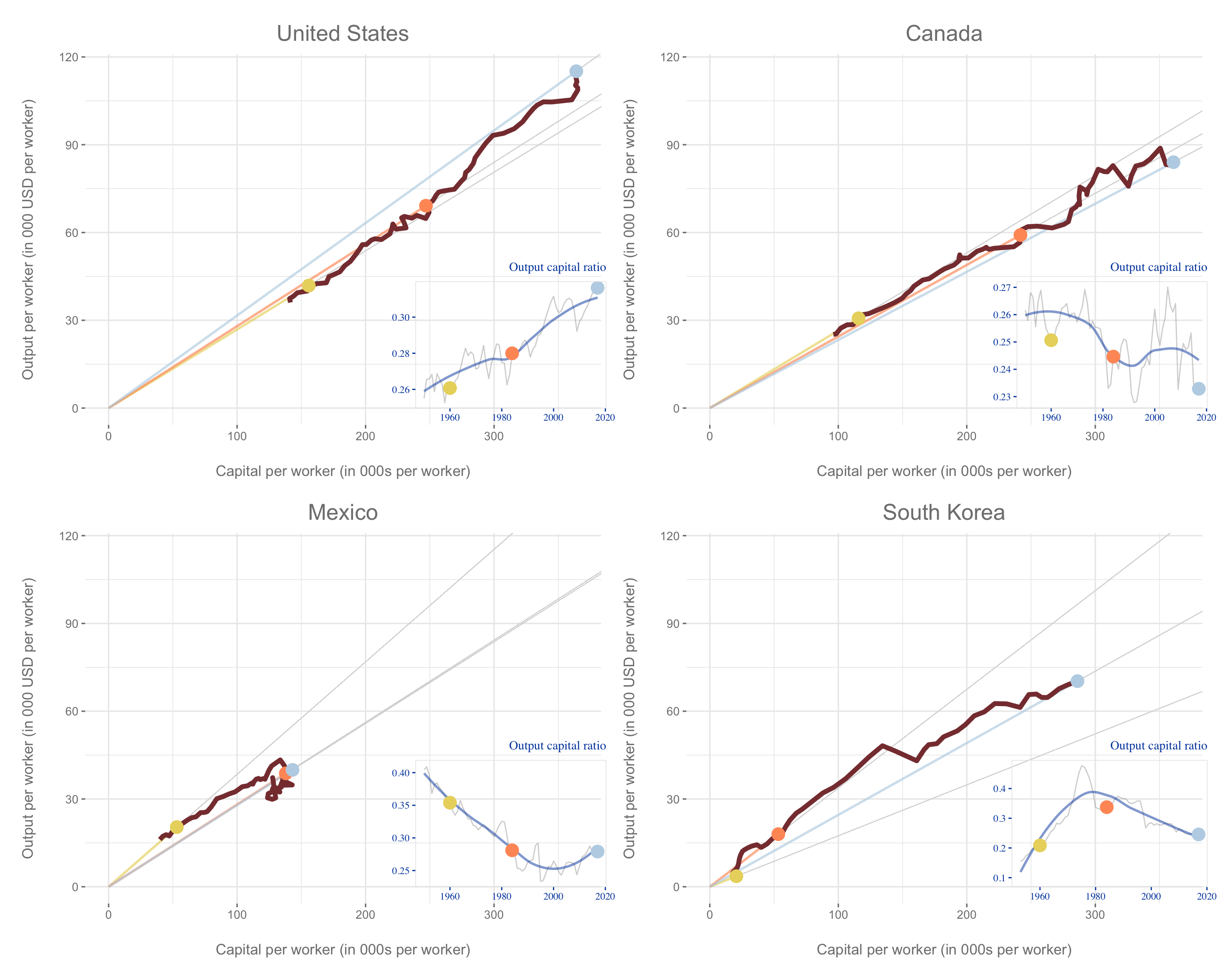
Figure 2.2: Production function and output-capital ratio
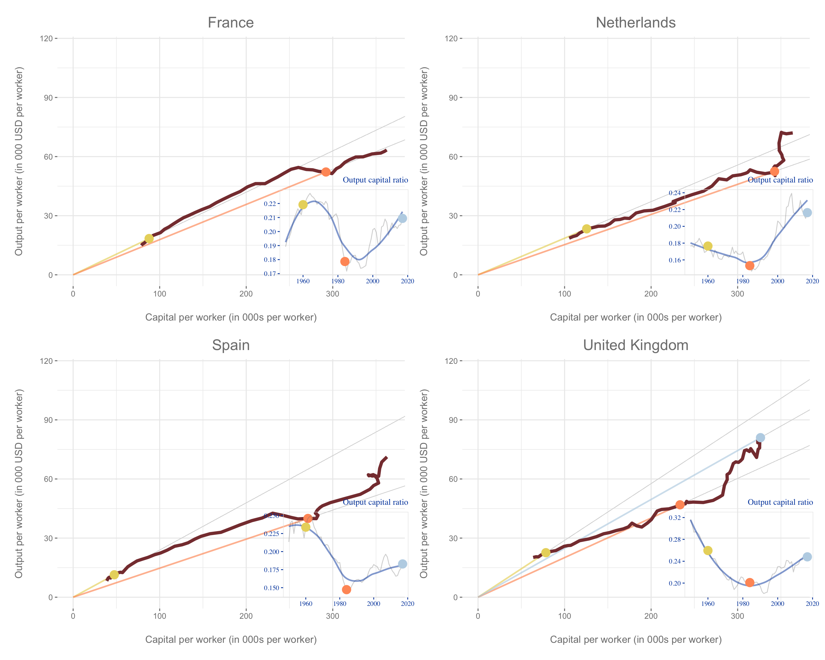
Figure 2.3: Production function and output-capital ratio
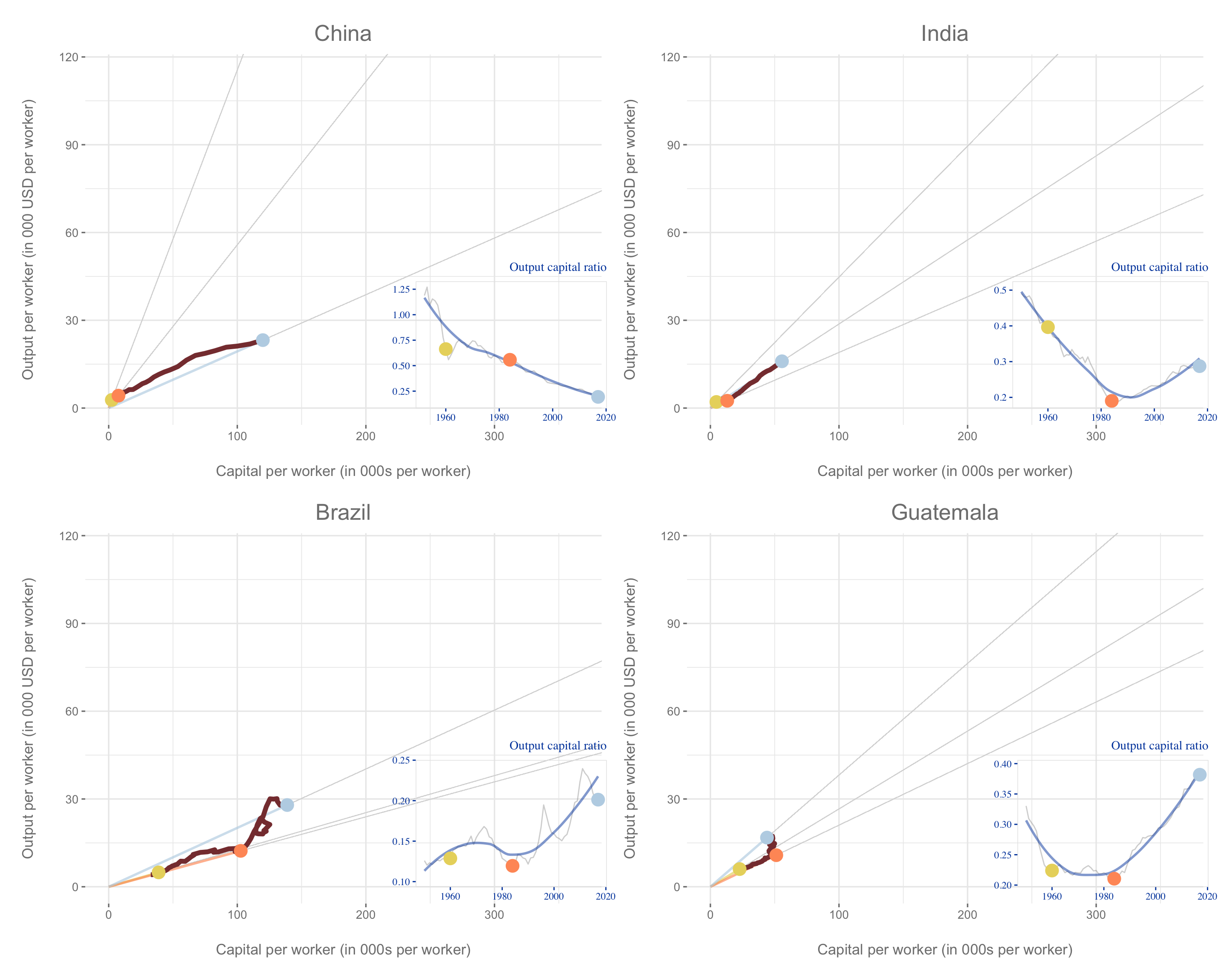
Figure 2.4: Production function and output-capital ratio
While Solow growth model was prevalent framework till 1980, the evidence of output-capital ratio increasing over time in certain countries was puzzling. While some evidence validated the Solow Growth model, there were also patterns that challenged it. It seemed to suggest that while Solow growth model did captured an essential phenomenon, there was some other phenomenon at work which needed investigation. This inspired Paul Romer and Robert Lucas to reexamine the neo-classical growth theory models and leds to birth of a new class of models called the endogenous growth theory.
2.4.1 Birth of Endogenous Growth Theory
To understand the endogenous growth theory, we would have think about what was the source of economic growth in Solow Growth model. In Solow Growth model, the output per-worker grew because capital per worker grew, i.e., the capital accumulation process.
What was the force that was driving the capital accumulation process? There were two distinct types of capital accumulation processes.
The first type was when the economy was at a distance away from its steady state and its savings was greater than depreciation. As a result, the firms in the economy accumulated capital as the economy converged to its steady state. The closer the economy got to its steady state, the slow the capital accumulation process got.
The second kind of capital accumulation process was the one that took place once the economy was in steady state. Once the economy was in steady, the capital accumulation was such that the capital per-effective worker would not change and leave the economy in steady state perpetually. This required just enough capital accumulation per period so that it matches capital lost to depreciation, capital allocated to new member entering the labour force and capital that matched the rise in labour productivity \(A\). While \(k=\frac{K}{AL}\) remains constant during steady state, it implies that capital per worker grows exactly at the rate of \(A\) to ensure that capital per effective worker remains constant. That is, \(g_k=\frac{\Delta{k}}{k}=0\) implies that \(g_{\left[\frac{K}{L}\right]}=\frac{\Delta{\left[\frac{K}{L}\right]}}{\left[\frac{K}{L}\right]}=\frac{\Delta{A}}{A}=g_A\).
This meant that the source of growth or capital accumulation in the steady in Solow Growth model is exogenous, i.e., not something explained by the model. While the neo-classical economic growth literature’s ability to identify capital accumulation process as the source of growth was a giant intellectual step, it still did not resolve the mystery of why some countries grew fast and others grew slowly. Put another way, if a country wanted to accelerate their economic growth, what policies would they have to put in place? Since \(A\) was not clearly identified in the model, the answer was not very clear.
To understand the exogenous nature of \(A\), we would have to distinguish between the theoretical modelling of \(A\) and empirical evidence of \(A\). From a theoretical perspective, \(A\) was modelled as the any set of ideas that increased the productivity of labour. From an empirical perspective, the output, capital stock and labour force in the economy were tangible quantities that could be observed and quantified from the national income accounts of a country. Conversely, \(A\) was intangible and it was impossible to quantify at the aggregate level for a country. The fact that it was intangible did not mean that it was not real. There seemed overwhelming evidence that it had a huge impact on the fortunes of nation and different nations had a different evolution of \(A\). So, the only was in which \(A\) could be estimated empirically was as the unexplained bit or the residual bit. Hence, it came to be known as Solow’s residual.
Cobb Douglas Production Function:
\[\begin{align} Y=K^\alpha {(AL)}^{1-\alpha} \end{align}\]
The relationship of rate at which the variables grow is as follows.
\[\begin{align} g_Y=\alpha{g_K} + (1-\alpha)g_L + q \end{align}\]
where \(q\) is the Solow’s residual, i.e., the change in \(Y\) that cannot be explained by the change in \(K\) and \(L\).11
These graphs allow us to examine whether the diminishing returns to capital assumption can be validated from evidence across the world. The slope of the line connecting the origin to the coloured dots give us the output-capital ratio. The evolution of output-capital ratio over time is also represented in the inset graphs. The evidence is mixed. While there are long period period where we observe the output-capital ratio decreases as capital per worker increases validating the assumption of diminishing marginal product of capital, there are also period where output per capital increases with as capital per worker increases, thus challenging the assumption.
the along with how their output-capital ratio has evolved over this period of time. We find that countries go through a distinct phases where the output-capital ratio is declining as diminishing marginal product of capital sets in and then other phases where the output-capital ratio sharply increases indicating either a sharp rise is \(A\) or some process that offsets the diminishing marginal product of capital.
2.5 Summary
This chapter explores the capital accumulation leads to economic growth in an economy. At its essence, an economy accumulates the non-consumed output in form of capital stocks12. It is the diminishing marginal returns to capital that ensures that the economy converges to a steady state. The steady state is determined by the parameters \(s,n,g\) and \(\delta\). In the steady state, capital per worker and output per workers grows as the same rate of \(A\). In the production \(Y=F(K, AL)\), \(A\) can be described as anything that makes workers more productive. Developing countries can increase their per-capita income or living standards by either increasing the rate at which \(A\) grows or ensuring the marginal product of capital is no longer diminishing.
\(A\) is a catch all term for everything impacts the workers’ productivity. In the next lecture, we wil explore what factors influence the growth rate of economy’s \(A\).